Integration involves finding a function based on its derivative (slope). This means that if the slope of a function is known, the function itself can be found. Sometimes this is done symbolically, with equations, but in chemistry it is usually done n umerically. If we can find the amount of change going on during a little bit of time at a lot of different times, these values can be summed, giving the total change over that time. Then that change is added to a known starting value to give an approxim ate ending value. "Integration" refers to the process of finding and adding up those small changes.

Integration can be thought of as finding the area under a curve. If that curve is a derivative, then the area under it for a given interval of x values is the same as the change in the original function over that interval. This process can also be used to solve differential equations, equations which represent the derivative of another function. If a starting value is specified and the differential equation is integrated over a given interval, that value is added or subtracted from the starting value to find the ending value.

In chemistry, this process is most often used when we are concerned with the course of a reaction over time. For example, it is possible to figure out how quickly each species in a reaction is changing if the reaction mechanism (the exact way it happe ns) and some simple data are known. This representation of how quickly the concentrations are changing is the same as a slope, or derivative. Integration allows us to find the actual change over time and not just how quickly the change is happening. 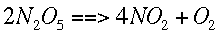Fo r example, given the following reaction,

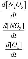
We can find how quickly each concentration is changing over time. This is symbolized by

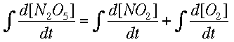
Now, integrating allows us to find the way the concentrations change, instead of the rate of change.

Numerical Methods

Integration can be done with equations, but chemists are usually more interested in real data, meaning numbers, than a symbolic integration (which can be quite tricky for some reactions). Numerical methods are used in these cases to approximate the ch ange in a concentration over time when the rate of change is known at several different times. Usually the rate of change is known from a reaction mechanism and some data.

Two major forms of numerical integration are used: Euler's method and Runge-Kutta methods. In this reading, we will examine Euler's method and briefly see a Runge-Kutta example.

Euler's Method

The basic idea behind Euler's method is to approximate a curve with a series of straight lines. The rate of change is the same as the slope of a line drawn tangent to the curve at that time. A series of these tangent lines can be used to "follow" th e function over time. An example is shown below.

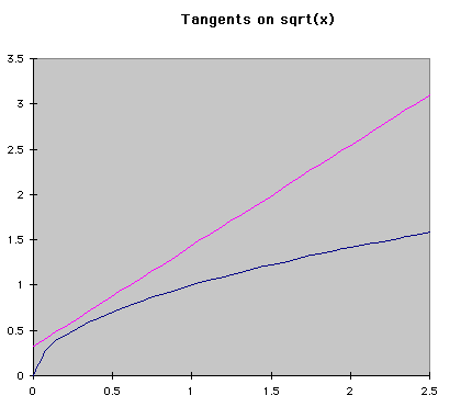
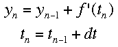
If f'(t) is the change over time at a given time, and a is the time when the tangent is being drawn, then the equation of a tangent line at any time is f'(t)*(t-a)+f(a).

Using the same idea, we can see that the following equations represent the change in y and time over a given space of time. Triangle t is read "delta t", which represents the step size being used. The subscripts represent the number of steps that hav e been taken so far. Using this process, Euler's method "steps" along the curve.

Integration Calculator based on Euler's Method

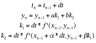
Runge-Kutta Methods

The Runge-Kutta methods use multiple different approximations to the next value of y and average them. The equations for the process with two approximations (Runge-Kutta 2 method) is shown below.

Back to:Mathematics Index

[Basic Matrix Math] [Linear Least Squares] [Newton's Method] [Integration Techniques]

Developed by

The Shodor Education Foundation, Inc.
in cooperation with the Department of Chemistry,
Appalachian State University