SCSI ADVANCED SESSION
JULY 16-22, 2000

TEAM MEMBERS
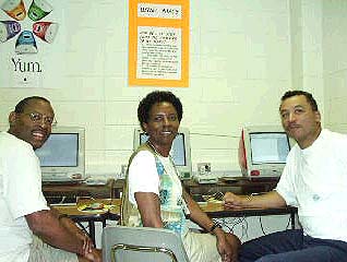
Douglas DePriest and Carolyn Morgan
Department of Mathematics
Morris Morgan
School of Engineering and Technology
SCSI ADVANCED SESSION
JULY 16-22, 2000

TEAM MEMBERS
Douglas DePriest and Carolyn Morgan
Department of Mathematics
Morris Morgan
School of Engineering and Technology
Two Problems:
Explore how Stella, Matlab and Maple can be used to model and solve a set of nonlinear ODEs (Ordinary Differential Equations) that describes the mass flow and temperature distribution in a mixing tank undergoing linear and nonlinear controls. The set of equations are conservation equations for mass and energy. The application represents a homework assignment problem given in the Hampton University Mathematics Department MAT 403 Numerical Analysis course and the School of Engineering and Technology EGR 307 Numerical Methods course. The results of the solutions obtained using the three computational science tools will be described and compared. Several graphical displays (including a phase plot and time plots) of the system mass and temperature are provided. Associated graphical displays allow the user to modify many of the important system input variables.
CASE 1: No trim heater - inlet mass flowrate disturbance
CASE 2: Trim heater with linear controller - inlet mass flowrate disturbance
Q = k * ( Tsp Ł T )
CASE 3: Trim heater with nonlinear controller - inlet mass flowrate disturbance
Q = k * ( Tsp Ł T ) 2
Where Q = heat flow, k = controller gain, Tsp = set point temperature, T = water temperature,
Also:
Explore how Stella, Matlab and Maple can be used to model and solve the following set of nonlinear ODEs (Ordinary Differential Equations):
These sets of equations are referred to as predator-prey equations. The application represents a homework assignment problem given in the Hampton University Mathematics Department MAT 403 Numerical Analysis course and the School of Engineering and Technology EGR 307 Numerical Methods course. The results of the solutions obtained using the three computational science tools will be described and compared. Several graphical displays (including a phase plot and time plots) of the prey and predator populations will be presented.