 Introduction to StellaAnne Thissen Stella is a dynamic modeling system in which you build models by creating a relational diagram and then assigning values and functions. First, every time you open up the program, find the little 'world' symbol in the lefthand toolbar and click it so it changes to an 'x squared' symbol. This will put you in the actual model-building layer. Otherwise you're just drawing and not really doing anything. There are several tools you'll want to use when you're creating a Stella model. Just click on them once in the menu bar and once in the model where you want them.
Connectors are the little pink arrows. They are links for values that need to be transmitted around a model, say, to and from converters. Click on the place you want the number to come from, and drag to where you want it to go to. The connector will follow.
ActivitiesFalling RockLet's begin with a relatively simple model. We will model the straight-down fall of a rock from rest at some height. For this we need only two dimensions: height and time. In Stella, one way to model it has height as a stock and downward motion as a flow. You have a certain amount of height to start with, and it flows out as gravity pulls the rock downward. So begin by making a stock called height and a flow coming out from it, downward velocity. All you need to tell Stella is the initial value for the stock, and the equation for the velocity. To do this, click on the stock. There's a big box at the bottom. Type in your initial height there (you can change it later) and ignore everything else for now. With the flow, you type in the equation in the same place (in this case 9.8 * time, unless you're using non-metric units). Note that Stella automatically subtracts an outward-pointing flow, so you do not need to make it negative. Now make a graph and put it somewhere. It doesn't matter where, just drop it on the paper somewhere convenient. Double click it. You should get a blank graph. Go under the Model menu to 'define graph'. Under 'Allowable' you should see a list like this:
Downward_Velocity Under the Run menu, go to 'Time Specs...' There's a list of different units of time to choose from, mostly more appropriate for medical or biological models than a falling rock. Choose 'Other' and type 'Seconds' in the box beside it. You can change the length of the simulation if you want to. DT should be about .25 for a start. We'll change that later. There's also a list of integration methods. Choose Euler's method. We'll also experiment with that later. Now go to your graph again and under the Run menu choose Run. The graph will appear for the rock's fall. Only... for some of you, no doubt the rock went right through the ground and far beyond it. Don't worry, that just happens. After all, we didn't include the ground in our equations, did we?
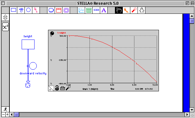
Go back into the main window and doubleclick on 'Height' again. Near the top there is a checkbox for 'Non-negative'. Click that and run your model again. Now we have a ground at zero. There is more than one way to make numerical integration more accurate. The first is to decrease the interval between approximations. Experiment with changing the size of DT (under Time Specs...). Does it change the result? Another way is to change the type of integration. Again under Time Specs, try one of the Runge-Kutta methods. Run your model again. Notice anything different? Notice anything wrong? The graph, right at the end, is leveling off. The rock not only doesn't go through the ground, it knows when the ground is coming and slows down! Well, maybe Euler's method is better after all? Actually, the Runge-Kutta methods are generally better. They just don't deal as well with discontinuities. When you made 'Height' non-negative, you created a discontinuity, a boundary condition. The Runge-Kutta methods try to match the Height function on either side of the discontinuity. Another way to look at it is that the Runge-Kutta methods are averaging iterations of a method like Euler's, over several steps. When the function reaches zero, the method begins averaging in zeroes, and this causes the function to approach the ground more gradually. So, for the Runge-Kutta methods to work, you have to de-select non-negative. But at least we don't have to _see_ where the rock goes belowground. Get back in your graph window and look under 'Define Graph'. Click once on 'Height' in the 'Selected' window, and once on the up-and-down arrows. This will give you boxes to set the scale. Set the bottom one to zero. Thrown RockWhat if the rock were not just dropped from a height, but tossed up into the air? It could have an initial height _and_ an initial velocity. Modify your dropped-rock model (you might want to save it first!) to include an initial velocity upwards. This could simply be a constant added onto the gravity-induced motion (think about this: would it be a _positive_ or _negative_ constant?), or you can make an in-flow on the other side of Height, with a constant value. When you run the model, you may find you need to reset your graph scale to accomodate the upward motion of the rock. Rocket ModelFor a more challenging model, let's try the ascent of a rocket. For this model, not only is work being done on the rocket as it flies, but we can't even use the simplified formula for acceleration that most of us are familiar with, acceleration = force / mass. In this case, force (dp/dt where p is momentum) is equal to the time derivative of mass times velocity:
F = ma + v(dm/dt) a = (F-v(dm/dt))/m This last equation is the one we will use. You will need to account for dm/dt twice. The rocket is losing fuel mass, which constitutes the majority of the mass of the rocket, and sections of the rocket are separating and falling away. You will create this model on your own. I suggest you create a second stock for velocity, with flows of its own, and a third for mass. The 'Become Graph' function of flows will be of use to you in this model. That allows you to change the relationship of two variables (say, dm/dt and time) over the span of one, by inputting pairs of values. Start by putting your independent variable (say, 'time') in the input box, as if it was a direct one-to-one relationship you were modelling. Then click 'Become Graph' at the bottom. You will probably want to change the number of data points (by clicking and typing in the box labelled that) and the range of the graph. Don't try to change the range by using the boxes next to the slider. That's just changing what you're looking at. Below them are two bigger boxes -- use those to set the minimum and maximum points. Now you can change individual values by clicking once on the 'input value' in the list and typing in the 'edit output' box. For a Saturn V (the big rockets that lifted the Apollo spacecraft), we will model the first, and part of the second, stage flights. Assume no air resistance and no change in gravity. You can use the following data:
Total mass (approx.) at liftoff:
First stage weight at liftoff:
     5.03 x 10^6 lbs = 2.29 x 10^6 kg
Weight of fuel burned in first stage:
     3,191,933 lbs LOX + 1,380,410 lbs kerosene = ()
Weight of fuel burned in second stage:
     812,352 lbs LOX + 154,266 lbs LH2 = ()

Rocket force:
First stage: 7.65 x 10^6 lbs = 3.41 x 10^7 N at liftoff
	rising to	9.16 x 10^6 lbs = 4.08x10^7 N by cutoff
Second stage: 1.156 x 10^6 lbs = 5.15 x 10^6 N

Ascent sequence:
T+0		launch
135		cut off first stage engines and coast
160		jettison first stage
165		second stage engines on
Simulation good for approximately 180 s. Data from a copy of the Saturn V Flight Manual posted in part to the Web by (Anne needs to find this), except for the total mass which is an approximation. Last update on: June 1, 1998 Please direct questions and comments about this page to WebMaster@shodor.org © Copyright 1998 The Shodor Education Foundation, Inc. |
 Stocks are containers. Use this where you have a value being changed, items being stored, a population, etc.
 Flows are changes over time (derivatives)
of stocks. Use it to represent when quantities from a stock enter or leave the system, or attach it to two stocks (by dragging from one to the other instead of clicking) to transfer a quantity from one to the other.
Flows are changes over time (derivatives)
of stocks. Use it to represent when quantities from a stock enter or leave the system, or attach it to two stocks (by dragging from one to the other instead of clicking) to transfer a quantity from one to the other.
 Converters hold constants, unit transformation equations, etc. They attach with connectors.
 This icon, when clicked, opens up a graph. What it's graphing is set under a menu, so you don't need to connect it anywhere.