


Angular Solution of Hydrogen Lesson
Lesson - Angular Solution of Hydrogen AtomSchrodinger's EquationSchroedinger's equation applied to a single electron Hydrogen atom takes the following form:
Written in terms of angular and radial portions, Schrodinger's equation is given by
where
Written in terms of the angular variables
Azimuthal Term
Noticing that the
In order for Y to be an eigenfunction of the angular momentum
equation, T must be an eigenfunction separately of the
The solution to this is clearly a combination of sine and cosine functions
which in its most general form is often written as
but what values of
In this case, T is a function of the angle
For what values of
Making a polar
plot of the sin and cosine functions, it is easy to see that
functions where
Polar TermPutting this back into the equation for angular momentum we get
Making the substitution
While this equation may not have an obvious solution, there are a few things we can see when looking at it.
The equation is not changed if the substitution
The equation has the potential to have singularities at
We cannot make the assumptions for boundary conditions that we did
with azimuthal angle
A
CSERD model of the Legendre Equation
exists which numerically solves this equation from
near -1 to near 1. (It will display as if it is solved from 1
to 1 because of the tool used to create the model.) This
model is being solved for units where The eigenvalues of this equation are often written as
Does this agree with your results? Like the radial solution for Shrodinger's equation applied to Hydrogen with one electron, this equation also can be solved exactly. For a derivation of the exact solution, please see MathWorld.
The solutions to the above equation with SolutionUsing this solution, and our assumptions about the periodicity of the azimuthal solution, we can write the solution to the angular portion of Schrodinger's equation for a single electron Hydrogen atom as
where
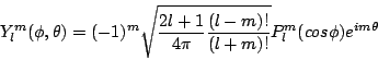
and for
The extra terms in the coefficient are strictly for normalization. Nothing in our solution to the equation specified the amplitude of the solutions, so they have been normalized according to standard conventions. The solution to the angular momentum equation are used often in physics, and are reffered to as the Spherical Harmonics. A description of the Spherical Harmonics can be found at MathWorld, including solutions for the first few terms. (From: p. 165, Brandt & Dahmen, The Picture Book of Quantum Mechanics, second edition 1995) Exercises |