| |
|
Gaussian Plume Model: Algorithm
The "standard" algorithm used in plume studies is the Gaussian plume model, develped in 1932 by O.G. Sutton. The algorithm is as follows:
 where:
- C(x,y,z) is the concentration of the emission (in micrograms per cubic meter) at any point x meters downwind of the source, y meters laterally from the centerline of the plume, and z meters above ground level.
- Q is the quantity or mass of the emission (in grams) per unit of time (seconds)
- u is the wind speed (in meters per second)
- h is the height of the source above ground level (in meters)
-
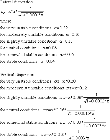
 and and  are the standard deviations of a statistically normal plume in the lateral and vertical dimensions, respectively are the standard deviations of a statistically normal plume in the lateral and vertical dimensions, respectively
This algorithm has been shown in a number of studies to be fairly predictive of emission dispersion in a variety of conditions. If you look at some of the examples on other Web links, you will find its application in roadside, urban, and long-term conditions. In this algorithm, we are concerned with dispersion in all three dimensions (x, y, and z):
- longitudinally (in the x direction) along a centerline of maximum concentration running downwind from the source
- laterally (in the y direction) on either side of the centerline, as the pollution spreads out sideways
- vertically (in the z direction) above and below a horizontal axis drawn through the source
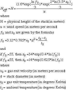
The other major calculations for a simple Gaussian plume model are as follows:
- Effective Stack Height:

- Lateral and Vertical Dispersion Coefficients:

- Ground-Level Concentrations:

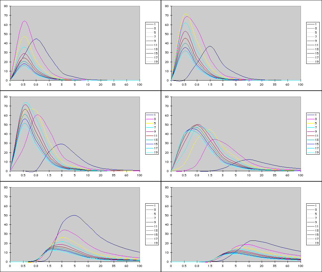
The stability categories were developed in the late 1970s, and are based on wind speed, insolation, and extent of cloud cover. As shown above, we can calculate the values the standard deviations from the downwind axis for these six conditions or categories using the algorithms above. The animated graphic below shows the effects of the downwind distribution of pollutant as a function of atmospheric stability. This animation begins with very unstable air, moving through the categories to stable air. On the x-axis is the distance downwind in kilometers, beginning at 0 and going to 100. On the y-axis is the concentration of pollutant in micrograms per cubic meter. Each of the six stability categories and the plume results is displayed in a continuous loop at one second intervals. You can run your own gaussian plume runs using the interactive models described on the next page:

Confused? Have a question? If so, check out the Frequently Asked Questions (FAQ) page or send mail to the OS411 tutor (os411tutor@shodor.org) with your question!
Report technical/content problems here
|
|

